Mastering continuous compound interest calculator principles
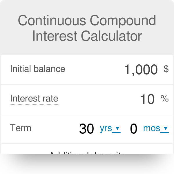
Table of Contents
- Mathematical Foundations of Compound Interest Calculators
- Exponential Growth Formula and Discrete Compounding
- Derivation of Continuous Compounding via Limits
- Comparison of Discrete and Continuous Compounding
- Effective Annual Rate (EAR) for Continuous Compounding
- Technical Implementation of Continuous Compounding in Financial Calculators
- Algorithmic Steps for Continuous Compounding Calculation
- Pseudocode for Continuous Compounding Function
- Common Programming Pitfalls and Solutions
- Computational Efficiency: Iterative vs. Direct Formulaic Approaches
- Applications of Continuous Compounding in Financial Instruments and Real-World Scenarios
- Role in Bond and Derivative Valuation
- Industries Relying on Continuous Compounding
- Comparison of Continuous vs. Discrete Compounding Scenarios
- Inflation-Adjusted Returns and Retirement Planning
- User Interface and Design Considerations for Continuous Compounding Calculators
- Essential UI Elements for Continuous Compounding Calculators
- Responsive HTML Table for Compounding Results Over Time
- Visualizing Continuous Growth Curves
- Accessibility Features for Inclusive Design
- Advanced Topics: Extensions and Variations of Continuous Compounding Models
- Modifications for Variable Interest Rates
- Inverse Problem: Solving for Rate or Time
- Alternative Compounding Models and Their Use Cases
- Integration with Time Value of Money and Net Present Value
- Educational and Demonstrative Use Cases for Teaching Continuous Compounding
- Step-by-Step Guide for Teaching Continuous Compounding to High School Students
- Dynamic Infographic: Comparing Continuous and Discrete Compounding Over 30 Years
- Command-Line Tool for Simulating Continuous Compounding
- Jupyter Notebook for Visualizing Continuous Compounding with Python
Understanding continuous compound interest transforms financial decision-making by revealing how investments grow exponentially over time without discrete intervals. This concept, rooted in mathematical precision, bridges theory and practical applications across finance, technology, and economics. By dissecting the exponential growth formula and its continuous counterpart, professionals and educators can optimize calculators, refine investment strategies, and demystify complex financial instruments like derivatives and pension funds.
The continuous compounding model eliminates periodic limitations, offering a more accurate reflection of real-world scenarios where interest is reinvested instantaneously. From algorithmic implementation in software to user-centric design in calculators, this framework ensures clarity, efficiency, and accessibility. Whether applied to high school education or advanced financial modeling, its principles empower users to visualize growth patterns, mitigate errors, and align strategies with long-term objectives.
Mathematical Foundations of Compound Interest Calculators
The exponential growth of compound interest forms the backbone of financial mathematics, enabling precise calculations for investments, loans, and savings. At its core, compound interest accounts for the reinvestment of accumulated interest, leading to accelerated wealth accumulation over time. Understanding its mathematical derivation—particularly the transition from discrete to continuous compounding—provides clarity on how financial instruments optimize returns. This section explores the exponential growth formula, its transformation into continuous compounding via limits, and the practical implications for real-world financial scenarios.
The foundational formula for compound interest with discrete periods is derived from iterative multiplication of principal by a growth factor. This formula serves as the basis for all compounding scenarios, including annual, monthly, or daily intervals. By examining its structure and applying calculus, the continuous compounding formula emerges as a limiting case, offering theoretical and practical advantages in financial modeling.
Exponential Growth Formula and Discrete Compounding
The general formula for compound interest with discrete compounding periods is expressed as:A = P \left(1 + \frac{r}{n}\right)^{nt}Where:
This formula accounts for the effect of compounding by dividing the annual rate r by n (the compounding frequency) and raising the result to the power of nt (total compounding periods). For example, monthly compounding (n = 12) applies the growth factor 12 times per year, amplifying returns compared to annual compounding (n = 1).
Derivation of Continuous Compounding via Limits
Continuous compounding arises from the mathematical limit where the compounding frequency n approaches infinity. As n increases, the term \(\left(1 + \frac{r}{n}\right)^{nt}\) can be rewritten using the definition of the exponential function with base e (Euler's number, approximately 2.71828). The transformation relies on the following steps:1. Express the growth factor in exponential form:
The term \(\left(1 + \frac{r}{n}\right)^n\) converges to e^r as n approaches infinity. This is a fundamental limit in calculus:
\lim_{n \to \infty} \left(1 + \frac{r}{n}\right)^n = e^r2. Apply the limit to the compounding formula:
Substituting into the discrete formula, the future value A becomes:
A = P \cdot e^{rt}Here, the exponent rt replaces nt, as continuous compounding effectively occurs instantaneously over time.
3. Mathematical justification using natural logarithms:
The equivalence can be derived by taking the natural logarithm of the discrete formula and applying L'Hôpital's rule or Taylor series expansion for \(\ln(1 + x)\) as x approaches 0. For small increments (\(\frac{r}{n} \to 0\)), the approximation \(\ln(1 + x) \approx x\) holds, leading to:
\ln\left(\left(1 + \frac{r}{n}\right)^{nt}\right) = nt \cdot \ln\left(1 + \frac{r}{n}\right) \approx nt \cdot \frac{r}{n} = rtExponentiating both sides yields the continuous compounding formula.
Comparison of Discrete and Continuous Compounding
The following table contrasts discrete compounding frequencies with continuous compounding, highlighting their formulas, growth rates, and real-world applications. Continuous compounding, while theoretically ideal, serves as an upper bound for returns in practical scenarios.| Compounding Type | Formula | Growth Rate (for r = 5%, t = 1 year) | Real-World Implications |
|---|---|---|---|
| Annual (n = 1) | \(A = P(1 + r)^t\) | 5.00% | Simplest form; used in basic loan/interest calculations. |
| Monthly (n = 12) | \(A = P\left(1 + \frac{r}{12}\right)^{12t}\) | 5.12% | Common in savings accounts and mortgages; higher returns than annual. |
| Daily (n = 365) | \(A = P\left(1 + \frac{r}{365}\right)^{365t}\) | 5.13% | Approximates continuous growth; typical in high-frequency financial instruments. |
| Continuous | \(A = Pe^{rt}\) | 5.13% (asymptotic limit) | Theoretical maximum; used in option pricing (Black-Scholes model) and advanced derivatives. |
Effective Annual Rate (EAR) for Continuous Compounding
The Effective Annual Rate (EAR) measures the actual interest earned or paid over a year, accounting for compounding. For continuous compounding, the EAR is derived by solving for the equivalent discrete rate that yields the same future value as the continuous formula.Given a nominal annual rate r compounded continuously, the EAR is calculated as:
EAR = e^r - 1Example Calculation (Nominal r = 5%):
1. Substitute r = 0.05 into the formula:
EAR = e^{0.05} - 1 \approx 1.051271 - 1 = 0.051271 (5.1271%)2. Comparison with Nominal Rate:
Practical Implications:
Technical Implementation of Continuous Compounding in Financial Calculators
The mathematical foundation of continuous compounding provides a robust framework for modeling exponential growth in finance, but its practical implementation in calculators demands careful attention to algorithmic design, input validation, and computational precision. Unlike discrete compounding, where periodic interest application introduces granularity, continuous compounding relies on the natural exponential function, requiring precise handling of floating-point arithmetic, edge cases, and time unit conversions. This section explores the algorithmic steps, pseudocode structure, common pitfalls, and computational trade-offs inherent in building a continuous compound interest calculator.
The core challenge lies in translating the theoretical formula \( A = P \cdot e^{rt} \) into a computationally efficient and numerically stable implementation. Input validation ensures robustness against invalid or edge-case values, while precision handling mitigates floating-point errors that can distort results, particularly for large time horizons (t). Below, the discussion dissects the implementation process, from validation logic to performance optimizations, while addressing pitfalls that arise in real-world deployments.
Algorithmic Steps for Continuous Compounding Calculation
The implementation of continuous compounding follows a structured sequence of operations to ensure accuracy and reliability. The primary inputs—principal (P), annual interest rate (r), and time (t)—must undergo validation before computation. The algorithmic pipeline includes:1. Input Validation and Sanitization
2. Precision Handling for Exponentiation
3. Formula Application
4. Output Formatting
Pseudocode for Continuous Compounding Function
Below is a pseudocode representation of a function `continuous_compounding(P, r, t)` that adheres to the outlined steps. Key operations—exponentiation, precision handling, and input validation—are highlighted for clarity.FUNCTION continuous_compounding(P, r, t):
// Input validation
IF P ≤ 0 THEN
RETURN ERROR("Principal must be positive")
END IF
IF r < 0 THEN
RETURN ERROR("Negative rates require explicit handling")
END IF
IF t < 0 THEN
RETURN ERROR("Time cannot be negative")
END IF
// Normalize time to years (example: t in months → t = t / 12)
t_normalized = t
IF time_unit ≠ "years" THEN
t_normalized = t / CONVERSION_FACTOR(time_unit)
END IF
// Edge cases
IF t_normalized = 0 THEN
RETURN P
END IF
IF r = 0 THEN
RETURN P // Linear growth: A = P + 0 = P
END IF
// Compute exponent with precision handling
rt = r t_normalized
IF rt > MAX_PRECISION_THRESHOLD THEN
USE HIGH_PRECISION_LIBRARY()
END IF
// Exponential calculation
A = P EXP(rt)
// Round to 2 decimal places for currency
RETURN ROUND(A, 2)
Key Operations Explained:
Common Programming Pitfalls and Solutions
Implementing continuous compounding introduces several pitfalls, primarily stemming from floating-point arithmetic, unit mismatches, and edge-case oversight. Below is a curated list of challenges and their mitigations, presented as a blockquote for emphasis:
- Floating-Point Precision Errors
Pitfall: For large rt values (e.g., r = 0.1, t = 1000), \( e^{rt} \) exceeds the representable range of standard floating-point types, leading to overflow or loss of precision.
Solution: Use arbitrary-precision libraries (e.g., Python’s `decimal` module with sufficient precision) or logarithmic transformations to rescale computations. For example, compute \( A = P \cdot 10^{rt \cdot \log_{10}(e)} \) to avoid direct exponentiation of large numbers.
- Incorrect Time Unit Handling
Pitfall: Mixing time units (e.g., t in months but r as an annual rate) without conversion introduces systematic errors. For instance, \( t = 24 \) months with r = 0.05 should yield \( rt = 0.05 \times 2 = 0.1 \), not 1.2.
Solution: Enforce unit consistency by normalizing all time inputs to a base unit (years) during input parsing. Validate user-provided units against a predefined set (e.g., years, quarters, days).
- Edge-Case Mismanagement
Pitfall: Failing to handle t = 0 or r = 0 explicitly can lead to incorrect results. For t = 0, the formula \( A = P \cdot e^0 = P \) must be enforced, while r = 0 reduces to linear growth (A = P).
Solution: Implement pre-checks for these conditions before exponentiation. For r = 0, return P directly without further computation.
- Catastrophic Cancellation in Subtraction
Pitfall: When computing differences between nearly equal exponential terms (e.g., \( e^{rt} - e^{rt - \epsilon} \)), floating-point subtraction can lose significant digits due to limited mantissa precision.
Solution: Avoid subtraction-based operations in continuous compounding. If auxiliary metrics (e.g., interest earned) require such calculations, use logarithmic identities or high-precision arithmetic.
- Library-Specific Quirks
Pitfall: Some programming languages or libraries (e.g., JavaScript’s `Math.exp`) have limited precision or edge-case behaviors (e.g., returning `Infinity` for large inputs).
Solution: Test with boundary values (e.g., rt = 709.78 for IEEE 754 double-precision limits) and fall back to alternative libraries (e.g., `math.exp` in Python vs. `Math.exp` in JavaScript).
Computational Efficiency: Iterative vs. Direct Formulaic Approaches
The choice between iterative and direct formulaic methods for continuous compounding impacts performance, particularly for large t values. Below is a comparative analysis of the two approaches, including trade-offs and use-case recommendations.The direct formula \( A = P \cdot e^{rt} \) is the de facto standard for continuous compounding due to its \( O(1) \) time complexity. However, iterative approximations (e.g., simulating
Applications of Continuous Compounding in Financial Instruments and Real-World Scenarios
Continuous compounding serves as a foundational mathematical framework in modern finance, particularly in instruments where time-value adjustments, risk modeling, and valuation require precise approximations of exponential growth. Unlike discrete compounding, which relies on periodic intervals, continuous compounding provides a theoretically sound basis for pricing financial derivatives, assessing long-term liabilities, and optimizing investment strategies under uncertainty. Its adoption in industries such as actuarial science, pension fund management, and quantitative trading reflects its ability to model real-world scenarios where compounding occurs instantaneously or over infinitesimal time frames.The mathematical elegance of continuous compounding—exemplified by the formula \( A = P \cdot e^{rt} \)—enables financial professionals to derive closed-form solutions for complex instruments, reducing computational complexity while improving accuracy. This approach is particularly critical in environments where small errors in valuation can lead to significant financial misalignments, such as option pricing under the Black-Scholes framework or the discounting of cash flows in inflation-adjusted retirement planning.
Role in Bond and Derivative Valuation
Continuous compounding underpins the valuation of fixed-income securities and derivatives by providing a consistent framework for discounting future cash flows. In bond markets, the yield-to-maturity (YTM) is often calculated using continuous compounding to reflect the true cost of borrowing over time, especially for long-duration bonds where discrete compounding assumptions introduce material discrepancies. For derivatives, such as swaps and futures, continuous compounding aligns with the assumption of frictionless markets and instantaneous arbitrage, a cornerstone of models like Black-Scholes for European options.Key applications include:
Bond Pricing: The present value of a bond’s coupon payments and principal is computed using the continuously compounded yield curve, ensuring consistency with market conventions for risk-free rates (e.g., LIBOR or SOFR). Option Pricing: The Black-Scholes model assumes continuous dividend yields and interest rates, enabling the derivation of option premiums via the partial differential equation \( \frac{\partial V}{\partial t} + \frac{1}{2}\sigma^2 S^2 \frac{\partial^2 V}{\partial S^2} + rS \frac{\partial V}{\partial S} - rV = 0 \), where \( r \) is the continuously compounded risk-free rate. Interest Rate Derivatives: Swaps and caps/floors rely on continuous compounding for forward rate agreements (FRAs) and the pricing of embedded options, as discrete adjustments would distort the hedging relationships. The use of continuous compounding in derivatives ensures that the no-arbitrage principle holds under the assumption of perfect markets, where transactions occur without transaction costs or delays.Industries Relying on Continuous Compounding
Several industries leverage continuous compounding due to its ability to model long-term financial obligations, risk exposure, and growth trajectories with high precision. The following sectors demonstrate critical dependencies on this methodology:
- Actuarial Science and Insurance: Actuaries use continuous compounding to project liabilities for annuities, life insurance policies, and pension funds. For example, the valuation of a perpetuity with continuous payments is given by \( PV = \frac{C}{r} \), where \( r \) is the continuously compounded discount rate. This approach simplifies the calculation of reserves and ensures solvency under stochastic interest rate environments.
- Pension Fund Management: Defined-benefit pension plans rely on continuous compounding to estimate the present value of future obligations, aligning contributions with projected liabilities. The International Accounting Standards Board (IASB) permits the use of continuously compounded discount rates for measuring pension liabilities, as it better reflects the economic reality of compounding over decades.
- Quantitative Trading and Algorithmic Finance: High-frequency trading (HFT) and proprietary trading firms use continuous compounding to model intraday returns and optimize portfolio rebalancing. The log-normal distribution of asset returns, derived from continuous compounding assumptions, underpins many statistical arbitrage strategies.
- Central Banking and Monetary Policy: Central banks, such as the Federal Reserve or the European Central Bank, employ continuously compounded rates for policy instruments like repo operations and forward guidance. The overnight indexed swap (OIS) curve, a key benchmark, is constructed using continuous compounding to reflect the true cost of short-term funding.
Comparison of Continuous vs. Discrete Compounding Scenarios
The choice between continuous and discrete compounding yields divergent results depending on the time horizon, frequency of compounding, and the magnitude of the rate. Below is a comparative table illustrating scenarios where the two methods diverge significantly:
Scenario Continuous Compounding Outcome Discrete Compounding Outcome (e.g., Annual) Key Difference Short-Term Investments (<1 year) \( A = P \cdot e^{0.05 \times 0.5} \approx P \cdot 1.0253 \) \( A = P \cdot (1 + 0.05) = 1.05P \) Discrete compounding overstates returns by ~2.4% for 6-month investments at 5% annual rate. Long-Term Investments (30+ years) \( A = P \cdot e^{0.07 \times 30} \approx 10.07P \) \( A = P \cdot (1 + 0.07)^{30} \approx 7.61P \) Continuous compounding yields ~32% higher growth due to exponential scaling over time. High-Frequency Trading (Intraday) Models returns as \( \ln\left(\frac{S_t}{S_0}\right) \sim N(\mu t, \sigma^2 t) \), capturing instantaneity. Discrete models (e.g., daily returns) introduce compounding errors for sub-second transactions. Continuous models align with stochastic calculus in derivatives pricing. Inflation-Adjusted Returns (Real Rates) Real return: \( r_{\text{real}} = \ln(1 + r_{\text{nominal}}) - \ln(1 + \pi) \), where \( \pi \) is inflation. Discrete approximation: \( r_{\text{real}} \approx \frac{r_{\text{nominal}} - \pi}{1 + \pi} \). Continuous adjustment is more accurate for multi-decade projections. Pension Liability Discounting Present value of \( \$1 \) million in 20 years at 3%: \( \frac{1,000,000}{e^{0.03 \times 20}} \approx \$553,686 \). Discrete: \( \frac{1,000,000}{(1.03)^{20}} \approx \$553,686 \) (negligible difference here, but diverges at higher frequencies). Critical for semi-annual or monthly compounding in actuarial tables. For investments exceeding 10 years, the difference between continuous and annual compounding can exceed 10%, highlighting the importance of methodology selection in long-term financial planning.Inflation-Adjusted Returns and Retirement Planning
Continuous compounding provides a robust framework for adjusting nominal returns to real terms, accounting for the erosive effects of inflation on purchasing power. In retirement planning, this distinction is critical, as even modest inflation rates (e.g., 2–3%) can significantly reduce the sustainability of retirement savings over 30+ years. The Fisher equation, extended via continuous compounding, expresses the relationship between nominal (\( r_{\text{nominal}} \)), real (\( r_{\text{real}} \)), and inflation (\( \pi \)) rates as:\[
r_{\text{nominal}} = r_{\text{real}} + \pi + \frac{r_{\text{real}} \cdot \pi}{1 + r_{\text{real}}}
\]However, for small \( r_{\text{real}} \) and \( \pi \), the approximation \( r_{\text{real}} \approx r_{\text{nominal}} - \pi \) is common, but continuous compound
User Interface and Design Considerations for Continuous Compounding Calculators
Continuous compounding calculators require a well-structured user interface (UI) to ensure accuracy, usability, and accessibility. The design must balance mathematical precision with intuitive interaction, particularly when visualizing exponential growth over time. Effective UI elements—such as input validation, dynamic result tables, and interactive growth curves—enhance user comprehension while adhering to accessibility standards. Below are key considerations for implementing a robust and inclusive calculator interface.
Essential UI Elements for Continuous Compounding Calculators
The core functionality of a continuous compounding calculator depends on clear, labeled input fields, real-time feedback, and formatted output. Users must input parameters such as principal amount, annual interest rate, and time period, while the calculator processes these values using the continuous compounding formula:
\[ A = P \cdot e^{rt} \]Input fields should include:
Where:
\( A \) = Final amount \( P \) = Principal amount \( r \) = Annual interest rate (in decimal) \( t \) = Time in years \( e \) = Euler’s number (~2.71828)
Principal Amount: A numeric field with optional currency formatting (e.g., `$` or `€`) and validation to reject negative values or non-numeric inputs. Annual Interest Rate: A percentage input with a slider for quick adjustments, ensuring values are converted to decimal form internally. Time Period: A numeric field with unit selection (years, months, or days) and conversion logic for non-yearly inputs. Compounding Frequency (if hybrid): A dropdown for discrete compounding (e.g., annually, monthly) alongside continuous compounding, with clear labeling to avoid confusion. Output should display:
Final Amount: Highlighted with currency formatting and optional breakdowns (e.g., total interest earned). Growth Curve: A dynamic graph (line or logarithmic scale) showing the exponential trajectory over time. Error Messages: Contextual alerts for invalid inputs (e.g., "Rate cannot exceed 100%") with actionable suggestions. Responsive HTML Table for Compounding Results Over Time
A structured table enhances transparency by displaying intermediate results, such as yearly or monthly breakdowns of continuous growth. Semantic HTML ensures accessibility and responsiveness across devices. Below is an example structure using ``, ``, and `` for clarity:```html
```
Yearly Growth Breakdown for Continuous Compounding Year Starting Balance Interest Earned (Continuous) Ending Balance 1 $10,000.00 $1,051.71 $11,051.71 Total Interest Earned $5,171.07 $15,171.07 Key Design Principles for the Table:
Semantic Markup: ``, ``, and `` improve screen reader navigation and data organization. Responsive Styling: CSS media queries adjust column widths for mobile devices, with `data-label` attributes for hidden labels on small screens. Dynamic Generation: JavaScript populates rows based on user inputs, recalculating values for each time increment. Accessibility Attributes: `aria-describedby` links the table to its caption, while `scope="col"` clarifies header associations. Visualizing Continuous Growth Curves
Exponential growth from continuous compounding is best visualized using logarithmic scales or interactive sliders to mitigate the rapid divergence of values. Design principles for effective visualization include:Logarithmic Scales
Log scales linearize exponential growth, making trends easier to compare. For example, a plot of \( A = P \cdot e^{rt} \) on a log-linear graph will appear as a straight line, where the slope represents the growth rate. Libraries like D3.js or Chart.js can render such graphs dynamically, with tooltips displaying exact values on hover.Interactive Sliders
Sliders allow users to adjust parameters (e.g., interest rate or time) in real time, updating the graph and table simultaneously. Example implementations:
Rate Slider: Ranges from 0% to 20% (adjustable) with a stepper for precise values. Time Slider: Displays a timeline (e.g., 1–30 years) with play/pause functionality to animate growth. Comparison Mode: Overlay discrete compounding (e.g., annually) against continuous compounding to highlight differences. Design Considerations for Clarity
Color Coding: Use distinct colors for axes, curves, and data points (e.g., blue for continuous, green for discrete). Annotations: Highlight key inflection points (e.g., where returns double) with labels or markers. Responsive Containers: Ensure graphs resize without distortion, using CSS `max-width` and `height: auto`. Accessibility Features for Inclusive Design
Accessibility ensures calculators are usable by individuals with disabilities, including visual, motor, or cognitive impairments. Key features include:Keyboard Navigation
Tab Order: Logical sequence for inputs (principal → rate → time → calculate). Focus States: Visible outlines or color changes for focused elements (e.g., ` Shortcut Keys: Assign actions (e.g., "Enter" to calculate) where applicable. Screen Reader Support
ARIA Labels: Associate inputs with descriptive labels (e.g., `aria-label="Annual interest rate in percent"`). Live Regions: Announce recalculated results (e.g., `aria-live="polite"`) to update screen readers dynamically. MathML or LaTeX: For formulas, use ` Visual and Motor Accessibility
High-Contrast Mode: Ensure text and UI elements meet WCAG contrast ratios (minimum 4.5:1). Adjustable Text: Support system font scaling without breaking layouts. Alternative Inputs: Provide text fields alongside sliders for users who cannot use a mouse. Cognitive Accessibility
Clear Error Messages: Avoid technical jargon; use plain language (e.g., "Please enter a valid number"). Progressive Disclosure: Hide advanced options (e.g., custom compounding frequencies) behind a toggle. Consistent Terminology: Use uniform labels (e.g., "Annual Rate" instead of "APR" or "Nominal Rate"). Testing and Validation
Automated Tools: Validate with axe DevTools or WAVE for accessibility violations. User Testing: Include participants with disabilities in usability evaluations. Keyboard-Only Workflow: Verify all functionality is accessible without a mouse. Advanced Topics: Extensions and Variations of Continuous Compounding Models
Continuous compounding provides a mathematically elegant framework for modeling exponential growth in financial instruments, but its applicability extends beyond static interest rate environments. Real-world financial scenarios often involve dynamic rates, stochastic processes, or hybrid compounding structures that require modifications to the foundational formula \( A = P e^{rt} \). This section explores extensions to the continuous compounding model, including adaptations for variable rates, inverse problem solutions, alternative compounding paradigms, and integrations with broader financial valuation techniques.
Modifications for Variable Interest Rates
The standard continuous compounding formula assumes a constant interest rate \( r \). In practice, rates may vary over time due to economic conditions, policy changes, or contractual terms. Two primary approaches accommodate this variability:1. Piecewise Continuous Compounding
When rates change at discrete intervals, the formula is adapted by segmenting the time horizon into intervals \( [t_0, t_1], [t_1, t_2], \dots, [t_{n-1}, t_n] \), each with a distinct rate \( r_i \). The future value \( A \) is computed as:\( A = P e^{r_1 (t_1 - t_0)} \cdot e^{r_2 (t_2 - t_1)} \cdots e^{r_n (t_n - t_0)} = P \exp\left(\sum_{i=1}^n r_i (t_i - t_{i-1})\right) \)This method preserves the continuous compounding principle while allowing for rate adjustments at predefined nodes.2. Stochastic Continuous Compounding
For rates modeled as stochastic processes (e.g., geometric Brownian motion in the Black-Scholes framework), the continuous compounding formula integrates a stochastic differential equation (SDE). The future value becomes a random variable:\( dA_t = A_t (r_t dt + \sigma_t dW_t) \), where \( W_t \) is a Wiener process.The solution involves Itô calculus, yielding a log-normal distribution for \( A \). This approach underpins derivative pricing models where volatility and drift are explicitly modeled.
Inverse Problem: Solving for Rate or Time
The continuous compounding formula \( A = P e^{rt} \) can be inverted to solve for either the rate \( r \) or the time \( t \), given a target amount \( A \). These derivations are critical for financial planning and option pricing.1. Solving for the Interest Rate \( r \)
Rearranging the formula for \( r \) yields:\( r = \frac{\ln(A/P)}{t} \)This expression is used in yield curve construction, where bond prices are inverted to derive zero-coupon rates. For example, a 10-year bond priced at 95% of par with a face value of 100 implies:\( r = \frac{\ln(100/95)}{10} \approx 0.0513 \) or 5.13% annually.2. Solving for Time \( t \)
The time required to reach a target amount \( A \) is:\( t = \frac{\ln(A/P)}{r} \)This is applied in retirement planning or investment horizons. For instance, to grow \$1,000 to \$2,000 at a 7% continuous rate:\( t = \frac{\ln(2)}{0.07} \approx 9.90 \) years.Alternative Compounding Models and Their Use Cases
While continuous compounding dominates theoretical finance, other models address specific scenarios where exponential growth assumptions may not hold. Below are key alternatives with their applications:
- Logarithmic Compounding
Used in scenarios where growth is bounded or subject to diminishing returns, such as biological growth or certain economic models. The formula \( A = P \ln(1 + rt) \) approximates saturation effects, though it lacks the mathematical tractability of exponential models.- Hyperbolic Compounding
Models scenarios with accelerating growth, such as viral marketing or early-stage technology adoption. The hyperbolic form \( A = P \left(1 + \frac{t}{k}\right)^n \) can be adapted for continuous limits, though it requires careful parameterization to avoid singularities.- Fractional Compounding
Extends continuous compounding to fractional time derivatives, useful in modeling memory effects (e.g., fractional Brownian motion in finance). The future value is expressed as:\( A = P E_{\alpha}(rt^\alpha) \), where \( E_{\alpha} \) is the Mittag-Leffler function and \( \alpha \in (0,1) \) controls the "memory" of the process.This is employed in rough volatility models for option pricing.- Discrete-to-Continuous Approximations
For high-frequency compounding (e.g., daily or hourly), the limit \( \lim_{n \to \infty} \left(1 + \frac{r}{n}\right)^{nt} = e^{rt} \) is used to approximate discrete compounding. This bridges theoretical continuous models with practical discrete implementations.Integration with Time Value of Money and Net Present Value
Continuous compounding can be unified with other financial concepts to create comprehensive valuation frameworks. Two key integrations are:1. Continuous Discounting in Net Present Value (NPV)
The NPV of a cash flow stream \( \{C_t\} \) under continuous compounding is:\( NPV = \int_0^T C_t e^{-rt} \, dt \)This integral form generalizes the discrete NPV formula and is used in project evaluation where cash flows are continuous (e.g., oil reserves, perpetual streams). For example, the NPV of a perpetual annuity \( C \) is:\( NPV = \frac{C}{r} \)2. Unified Framework for Time Value of Money (TVM)
Combining continuous compounding with inflation-adjusted rates yields a real TVM model. If \( r \) is the nominal rate and \( \pi \) the inflation rate, the real rate \( r_{\text{real}} \) is approximated as:\( r_{\text{real}} \approx r - \pi \) (for small \( \pi \)), or more accurately via the Fisher equation:The future value in real terms becomes:
\( 1 + r = (1 + r_{\text{real}})(1 + \pi) \).\( A_{\text{real}} = P e^{r_{\text{real}} t} \)This is critical for cross-border investments or long-term planning where purchasing power parity matters.
Educational and Demonstrative Use Cases for Teaching Continuous Compounding
Continuous compounding serves as a powerful pedagogical tool to illustrate exponential growth, mathematical modeling, and real-world financial applications. High school students benefit from interactive and visual demonstrations that bridge abstract concepts with tangible analogies, while educators can leverage dynamic tools to reinforce understanding. This section provides structured teaching methods, visualization techniques, and computational exercises to engage learners effectively.
Step-by-Step Guide for Teaching Continuous Compounding to High School Students
Analogies and Conceptual Foundations
To introduce continuous compounding, begin with relatable analogies that emphasize exponential behavior. For example:
Bacterial Growth: A single bacterium divides every hour. In discrete compounding, growth occurs at fixed intervals (e.g., every hour). In continuous compounding, divisions happen instantaneously, accelerating growth exponentially over time. Population Expansion: Compare a town’s population growth with annual vs. instantaneous immigration rates. Interactive Exercises
1. Hands-On Simulation with Discrete vs. Continuous Models
Provide students with a spreadsheet or calculator to compute compound interest for: Annual compounding (e.g., 5% per year). Monthly compounding (5%/12 per month). Continuous compounding (using the formula \( A = P e^{rt} \)). Observe how the effective rate converges toward the continuous limit as compounding frequency increases. 2. Real-World Scenarios
Investment Growth: Compare a $1,000 investment at 10% annual interest under: Annual compounding: \( A = 1000 \times (1.10)^t \). Continuous compounding: \( A = 1000 \times e^{0.10t} \). Radioactive Decay: Introduce the inverse process (decay constant \( \lambda \)) to show how continuous models apply to non-financial phenomena. 3. Graphical Comparison
Plot both discrete and continuous growth curves on the same axes for \( t = 0 \) to \( 30 \) years. Highlight how the continuous curve smooths the jagged discrete steps. Key Formula Recap
For continuous compounding, the future value \( A \) is calculated as:
\[ A = P \times e^{rt} \]
where:
\( P \) = principal amount, \( r \) = annual interest rate (as a decimal), \( t \) = time in years, \( e \) ≈ 2.71828 (Euler’s number). Dynamic Infographic: Comparing Continuous and Discrete Compounding Over 30 Years
Design Components and Descriptions
The infographic should visually contrast the two compounding methods using the following elements:1. Axes and Time Scale
X-axis: Time in years (0 to 30), labeled with major ticks at 5-year intervals. Y-axis: Growth factor (ratio of \( A/P \)), logarithmic scale to accommodate exponential growth (e.g., 1 to \( e^{3} \approx 20.0855 \)). 2. Curves and Annotations
Discrete Compounding (Annual): Step function plotted at integer years (e.g., \( (1 + r)^1, (1 + r)^2, \dots \)). Label each step with the formula \( A = P(1 + r)^t \). Continuous Compounding: Smooth exponential curve \( e^{rt} \). Annotate key points (e.g., at \( t = 10 \), \( A/P = e^{10r} \)) with numerical values. Convergence Point: Highlight where the discrete steps approach the continuous curve (e.g., after 20–30 years for high \( r \)). 3. Legend and Formula Bar
Include a legend distinguishing the two methods with icons (e.g., a staircase for discrete, a smooth wave for continuous). Display the formulas side-by-side: Discrete: \( A = P(1 + \frac{r}{n})^{nt} \)
Continuous: \( A = Pe^{rt} \) 4. Interactive Elements (Digital Version)
Sliders to adjust: Interest rate \( r \) (e.g., 5% to 20%). Compounding frequency \( n \) (annual, monthly, daily). Real-time updates to show how increasing \( n \) makes the discrete curve approach the continuous limit. Example Data Points for 10% Annual Rate
Year Discrete (Annual) \( A/P \) Continuous \( A/P \) 5 1.6105 1.6487 10 2.5937 2.7183 20 6.7275 7.3891 30 17.4494 19.0855 Command-Line Tool for Simulating Continuous Compounding
Tool Overview
A Python script using the `math` library allows users to input parameters and compute continuous compounding results. The tool includes validation for inputs and formats output for clarity.Script Implementation
import math
import sysdef continuous_compounding():
print("Continuous Compounding Calculator")
print("-----------------------------------")try:
principal = float(input("Enter principal amount ($): "))
rate = float(input("Enter annual interest rate (%): ")) / 100
time = float(input("Enter time in years: "))
except ValueError:
print("Error: Invalid input. Use numeric values.")
sys.exit(1)if principal <= 0 or rate < 0 or time < 0:
print("Error: Principal, rate, and time must be positive.")
sys.exit(1)amount = principal math.exp(rate time)
effective_rate = (amount / principal) (1 / time) - 1print("\nResults:")
print(f"Future Value: ${amount:.2f}")
print(f"Effective Annual Rate: {effective_rate 100:.4f}%")if __name__ == "__main__":
continuous_compounding()Input/Output Examples
1. Example 1: Standard InvestmentEnter principal amount ($): 1000
Enter annual interest rate (%): 7
Enter time in years: 10Future Value: $1967.15
Effective Annual Rate: 7.2507%2. Example 2: High-Rate Scenario
Enter principal amount ($): 5000
Enter annual interest rate (%): 15
Enter time in years: 5Future Value: $12336.80
Effective Annual Rate: 16.0556%Error Handling
Rejects non-numeric inputs (e.g., text for rate). Validates positivity of inputs (e.g., time cannot be negative). Jupyter Notebook for Visualizing Continuous Compounding with Python
Setup and Dependencies
Install required libraries via pip:pip install numpy matplotlib jupyter
Notebook Structure
1. Imports and Configurationimport numpy as np
import matplotlib.pyplot as plt
%matplotlib inline2. Data Generation
Define parameters and compute values:P = 1000 # Principal
r = 0.05 # Annual rate (5%)
years = np.linspace(0, 30, 100) # Time array# Discrete (annual) compounding
discrete = P (1 + r) years# Continuous compounding
continuous = P np.exp(r years)3. Visualization Code
plt.figure(figsize=(10, 6))
plt.plot(years, discrete, 'b--', label='Annual Compounding')
plt.plot(years, continuous, 'r-', label='Continuous Compounding')
plt.title('Growth Comparison: Discrete vs. Continuous Compounding')
plt.xlabel('Years')
plt.ylabel('Amount ($)')
plt.axhline(y=P, color='k', linestyle=':', label='Principal')
plt.legend()
plt.grid(True)
plt.show()4. Interactive Plot with Sliders (Optional)
Use `ipywidgets` to allow dynamic adjustments:Continuous compound interest is not merely a mathematical abstraction but a dynamic tool that reshapes financial literacy and investment outcomes. By mastering its foundations—from exponential formulas to real-world applications—users gain the ability to design precise calculators, navigate complex financial instruments, and communicate growth scenarios with clarity. This synthesis of theory, implementation, and user experience underscores why continuous compounding remains indispensable in modern finance, education, and technological innovation.

Leave a Comment
Comments are moderated before appearing. The data you submit is processed according to the Privacy Policy of www.linuxunplugged.com.